A few months ago me and my friend decided to work on a project that breaks annoying captchas in course registration website. It was a fun project and a nice opportunity to put our knowledge into a real-world example. Throughout the process we have learned a lot, so I decided to write a tutorial that breaks down the steps we took. I hope this helps someone out there with a similar goal and if you have any suggestions feel free to contact.
Repo for this project is HERE.
Tools
To accomplish our goal we used python(3) and following libraries;
- opencv and numpy are used in image processing i.e. denoising the images and separating the digits.
- pytorch used for training the model that will autonomously breaks captchas.
Creating the Dataset
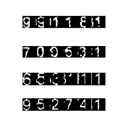
The very first step of the project is to create a dataset to work on with. Since we wanted to break a specific website’s captchas, we downloaded thousands of sample images via a click bot. Click bot basically refreshed the page and downloaded the captcha to a folder every time. We could have as many samples we want but decided that around five thousand would be enough in our purpose.
You can download the dataset HERE.
After constructing the dataset, here comes the crucial part. Annotating the dataset:). In every supervised learning problem, we have to annotate(label) our dataset, and I should admit it was the most boring part of the whole thing. Thankfully we had a saint friend who helped us with this task. Our labels for the dataset is a plain text file and every line has the solution for associated captcha image. For example line 15 in the text contains solution for “15.jpeg” image in the dataset.
You can download the labels HERE.
Denoising and Separating the Digits
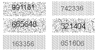
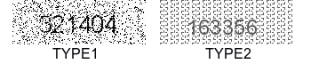
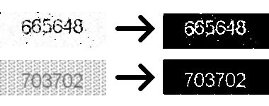
After creating our dataset we can experiment on it. At the first glimpse, you can see there are two different types of images. One seems to have a Gaussian noise and another one with periodical noise. We call them type1 and type2 images.
So the first image processing task should be determining the type of the given image, and then we can apply denoising on them with an intention to
separate digits clearly. Separating the digits is a necessity because we can only train our model based on the digits and not the whole images.
The gif below is a summary of denoising and separation steps.
To determine the type of image we need a general method that distinguishes between types. In this step, one could find multiple solutions that would work fine.
Our approach was based on image histograms. We saw that type 1 images contain lots of pure black(0 intensity value) in it, so a threshold value
for black pixel count actually worked perfectly.
def whichPattern(image):
	hist = cv2.calcHist([image], [0], None, [256], [0, 256])
	# pattern1 images has almost more than 600 pixels
	# for 0(pure black) intensity, lets set threshold to 500
	thresh = 500
	if(hist[0, 0] > thresh):
		return 1
	else:
		return 2
Above function takes an image as input and determines its type based on its histogram. The solution seems to be naive but works perfectly in this case. This link provides more information on calcHist function.
The whole point of determining the type was applying an appropriate filter to the image. It has seen that different filters work better on different types. After investigating couple image processing filters we decided on using median filter for type 1 and gaussian filter for type 2. Both of these filters smoothen images for further processing.
# use median blur for pattern1 and gaussian blur for patter2 images as pre-processing
srcImage = cv2.medianBlur(srcImage, 3) if pattern == 1 else cv2.GaussianBlur(srcImage, (3,3), 0)
You can find more about medianBlur and GaussionBlur here.
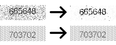
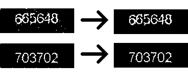
As we can see in Figure 3, smoothing filters make a great job at reducing the noise (especially for type1), therefore, now we can try binary threshold
to separate content(digits) from the background.
#obtained through experiment
pattern1_thresh = 170
pattern2_thresh = 155

thresh = pattern1_thresh if pattern == 1 else pattern2_thresh
ret, threshImage = cv2.threshold(srcImage, thresh, 255, cv2.THRESH_BINARY_INV)
Above code uses OpenCV’s threshold function to separate background and foreground of the images. Binary thresholding is one of the simplest method for image segmentation and very straight forward. It compares every pixel with a certain threshold value, then if the value of the pixel is less then the threshold it sets pixel’s intensity value to 0. In our case (see Fig 3.) digits actually have less intensity values than background so using inverse binary thresholding was appropriate. In this case, pixel values greater than the threshold set to 0(background) and remaining pixels set to 255(foreground). Each type has its own threshold value and these values selected based on manual inspection of sample images.
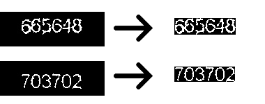
In Figure 4 we can see thresholding operation gives a binary image that only has black and white pixels. The type2 image seems be completely
noise free but the type1 image still has white pixel regions that are not part of the digits. Note that these regions relatively smaller than digits.
To delete this noisy parts we can use connected components.
min_connected_len = 15

# get connected components
numLabel, labelImage, stats, centroids = cv2.connectedComponentsWithStats(threshImage, 8, cv2.CV_32S)

# holds if component will be included to foreground
foreComps = [i for i in range(1, numLabel) if stats[i, cv2.CC_STAT_AREA] >= min_connected_len]

# Get binary image after erasing some connected components those areas under the threshold
binaryImage = np.zeros_like(srcImage)
labelImage = np.array(labelImage)
for k in [np.where(labelImage == i) for i in foreComps]:
	binaryImage[k] = 255
Using OpenCV’s connectedComponentsWithStats function we can find threshImage’s connected components with stats associated with it.
We have used 8-connectivity in order to
find connected components of the image. Here, labelImage is a matrix same size with the threshImage where each pixel of the certain connected component has the value of its own label
(0 being the background) and numLabel is the number of connected components. Knowing the labels of connected components we can choose those have areas(number of pixels) greater
than the min_connected_len thanks to CC_STAT_AREA. Finally, labels in foreComps are added to the foreground in binaryImage and other labels discarded(added to background).
From Figure 5, we can see connected component analysis made a great job at deleting regions that are not part of the digits. Now we can clip a rectangle that only contains the digits
thus removing the unnecessary background. In order to do that we need to find where do the digits lay in the image.
minCol = 30; # seen that all digits start at 30th column
			# no need for additional computation

# find the boundaries where digits present in the image
array = np.array([stats[i, cv2.CC_STAT_LEFT] + stats[i, cv2.CC_STAT_WIDTH]  for i in foreComps])
maxCol = max(array[np.where(array < 125)]) # observed that digits right boundary never exceeds 125th pixel
									# thus this one prevents false boundaries
# find boundaries in y axis
minRow = min([stats[i, cv2.CC_STAT_TOP] for i in foreComps])
maxRow = max([stats[i, cv2.CC_STAT_TOP] + stats[i, cv2.CC_STAT_HEIGHT] for i in foreComps])

subImage = threshImage[minRow:maxRow, minCol:maxCol]
Examining the dataset we saw left boundary of digits starts at 30, so minCol is fixed. Right boundary(maxCol) is the rightmost pixel in the foreground. This is found by
adding CC_STAT_LEFT and CC_STAT_WIDTH which is adding leftmost pixel of the connected component to its width. There is a little hack (np.where(array < 125) to prevent false boundaries that occurs
when some noise remained in the image. Upper and lower boundaries are found by similar manner.
So now we are close to ending of pre-processing, separating digits individually.
# Sub image divided to half in order to segment digit's more precisely
subImage1 = subImage[:, :int(subImage.shape[1]/2)]
subImage2 = subImage[:, int(subImage.shape[1]/2):]

colIncrement1 = subImage1.shape[1] / 3
colIncrement2 = subImage2.shape[1] / 3

# get segmented digits as list
digitList1 = []
digitList2 = []

col1 = 0
col2 = 0
for i in range(2):
	digitList1.append(subImage1[:, int(col1):int(col1+colIncrement1)])
	digitList2.append(subImage2[:, int(col2):int(col2+colIncrement2)])
	col1 += colIncrement1
	col2 += colIncrement2

digitList1.append(subImage1[:, int(col1):])
digitList2.append(subImage2[:, int(col2):])
digitList = digitList1 + digitList2
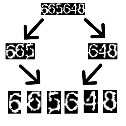
We could divide resulting subImage to 6 pieces of equal lengths in order to obtain separated digits. But it has seen that instead of dividing by six right away,
first dividing the image to half and then taking digits gives better results. Above code implements this approach. It first divides the image to half then
each half again divided to three to obtain digits. Results stored in digitList. You might wonder why we just didn’t take remaining connected components as digits.
Well, actually we couldn’t, because as we can see from Fig7 sometimes there is a gap between a digit’s parts(more than 6 connected components), and sometimes digits are touching each other(less than 6 connected
components).
Thus we achieved digit separation we could finish pre-processing here and start training our DL model. But when we checked some images we saw
that some parts of the digits shifted to other digits.
Although this phenomenon was rare and most of the images was correctly separated, we wanted to make something about it.
# It is observed that sometimes part of the previous digit shifted to
# digit that follows it.
# Following prevents it most of the time
for i in range(1, 6):
	# Appy slight closing before finding c.c, sometimes particular digit parts only apart by 1 pixels (fill them to avoid false shifting)
	kernel = cv2.getStructuringElement(cv2.MORPH_CROSS, (3,3))
	closedDigit= cv2.morphologyEx(digitList[i], cv2.MORPH_CLOSE, kernel, 1)

	numLabel, labelImage, stats, centroids = cv2.connectedComponentsWithStats(closedDigit, 8, cv2.CV_32S)
	if numLabel > 2: # consider shifting if there is more than 1(with background its 2)  c.c. per digit
		for j in range(1,numLabel):
			# If it touches left border of the image
			# and it's width doesnt exceed 35 percent of the digit, assume it is a shifting
			if stats[j, cv2.CC_STAT_LEFT] == 0 and stats[j, cv2.CC_STAT_LEFT] + stats[j, cv2.CC_STAT_WIDTH] < 0.35 * digitList[i].shape[1]:
				# find the part that will attach to previous digit
				startCol = stats[j, cv2.CC_STAT_LEFT]
				width_shifted = stats[j, cv2.CC_STAT_WIDTH]
				shiftedPart = digitList[i][:, startCol:startCol+width_shifted]

				# shift previous image to left while maintain its size
				# shift amount is width of the shifted-part
				fixedDigit = np.zeros_like(digitList[i - 1])
				fixedDigit[:, 0:fixedDigit.shape[1] - width_shifted] = digitList[i - 1][:, width_shifted:fixedDigit.shape[1]]

				# appending shifted part back to previous digit
				fixedDigit[:, fixedDigit.shape[1]-width_shifted:fixedDigit.shape[1]] = shiftedPart[:]

				digitList[i - 1] = fixedDigit # replace digit with fixed digit

				# remove shifted part from current digit
				digitList[i][:, 0:width_shifted] = 0
Ok. This one seems to be complex, but the idea is very simple. For better understanding let’s take a look at Fig9.

Hmm, first 9’s end is shifted to the second nine, second 9’s end is shifted to 1… and so on. Fixing this can be achieved by re-shifting the digit parts to the left.
To do that, first, we need to define rules for wrong shifting then take action. The very first thing we need to consider is if there are more than one connected components per separated digit.
(if numLabel > 2). This might be true because of shifting or there could be gaps between single digit parts(in Fig7, separated 5 has two c.c). So by only this fact we cannot conclude on wrong shifting exists.
Second thing to consider is shifted part need to always touching to left boundary of the digit image(if stats[j, cv2.CC_STAT_LEFT] == 0). In addition to that it is assumed shifted part is
no more than %35 of the image(stats[j, cv2.CC_STAT_LEFT] + stats[j, cv2.CC_STAT_WIDTH] < 0.35 * digitList[i].shape[1]). If the conditions satisfied then shifting to the left is applied.
Let’s see this in action in Gif2.
We did our best for separating digits. There might still bad separations but it will be enough to train our DL model.
Training the Model
Now we can define our model which is going to be trained on our dataset. For this task CNN’s are a great choice, they are the kings of image recognition.
import torch.nn as nn
import torch.nn.functional as F

class Net(nn.Module):
    def __init__(self):
        super(Net, self).__init__()
        # convolutional layer (sees 24x14x1 image tensor)
        self.conv1 = nn.Conv2d(1, 3, kernel_size=3)
        # convolutional layer (sees 22x12x3 tensor)
        self.conv2 = nn.Conv2d(3, 3, kernel_size=3)
        # linear layer (20 * 10 * 3 -> 30)
        self.fc1 = nn.Linear(20*10*3, 30)
        # linear layer (30 -> 10)
        self.fc2 = nn.Linear(30, 10)
    def forward(self, x):
        # sequance of convolutional layers with relu activation
        x = F.relu(self.conv1(x))
        x = F.relu(self.conv2(x))
        # flatten the image input
        x = x.view(-1, 20*10*3)
        # 1st hidden layer with relu activation
        x = F.relu(self.fc1(x))
        # output-layer
        x = self.fc2(x)
        return x
We are not experienced in NN architecture, but we know how to google :D. Pytorch provides a great example in image recognition so we were basically
playing with the parameters. Let’s quickly go over the model. The model contains two convolutional layers and two fully connected layers. First convolutional layer (self.conv1) expects
24x14x1 image tensor, here 24 and 14 are height and width of the image while 1 is the number of channels in the image(our images are grayscale thus 1 channel).
But why 24x14? Pytorch’s Conv2d excepts images with a fixed shape, i.e. all input images should have the same height and width.
To fix all digits shape before feeding them to model, we calculated the mean height and width of the images, and here comes the 24x14.
I believe the second important thing to mention here is figuring out correct parameters for the first fully connected layer. As you can see from the code it takes 20 * 10 * 3 as input tensor’s size.
We started with 24x14x1 but why end up with 20x10x3 tensors in convolutional layers? The reason is every time we go through a convolutional layer it shrinks the input size according to
applied kernel size in the absence of padding. Thus we are applying 3x3 kernel, it shrinks input tensor by 1 from the top, bottom, left and right. So conv1 gives 22x12x3 tensor as output and
conv2 gives 20x10x3 as its output. You can find more about the topic here.
Now we are ready to train our model. Let’s look at the train.py.
# Resize the images and convert to tensors
transform = transforms.Compose([transforms.Resize((24,14)),
            transforms.Grayscale(num_output_channels=1),
            transforms.ToTensor()])
Before loading the dataset we need to define the transforms that will apply to each image in the dataset. Here Resize function changes the size of the images to 24x14 for the
reason we mentioned above. Grayscale transforms images to grayscale and ToTensor converts the images to tensor so we could make computations on them.
# loads dataset from folder named train
# modify this path if you will load from other file
dset = datasets.ImageFolder(root='train', transform=transform)
dloader = torch.utils.data.DataLoader(dset,
    batch_size=8, shuffle=True, num_workers=12)
Pytorch’s datasets.ImageFolder lets us load datasets from folders. It expects a root path that contains
folders for each classification type (0..9 digits in this case). In the repository we have saveDigits.py python script to handle this. It uses the digit separation algorithm and labels
to save digits in their associated folders. I will show how to use it in a second.
# specify loss function (categorical cross-entropy)
criterion = nn.CrossEntropyLoss()
# specify optimizer
optimizer = optim.SGD(net.parameters(), lr=0.001, momentum=0.9)

n_epochs = 20
for epoch in range(n_epochs):
    running_loss = 0.0
    for i, (inp, lab) in enumerate(dloader, 0):
        inp = inp.to(device)
        lab = lab.to(device)

        # clear the gradients
        optimizer.zero_grad()
        # forward pass
        outs = net(inp)
        # batch loss
        loss = criterion(outs, lab)
        # backward pass
        loss.backward()
        # perform optimization(parameter update)
        optimizer.step()

        running_loss += loss.item()
        if i % 100 == 99:
            print('[%d, %d] loss: %f' % (epoch + 1, i+1, running_loss))
            running_loss = 0.0
print('finished')
torch.save(net.module if multi_gpu else net, 'model.pt')
Here, before running into the training loop, we define our loss function and optimizer to update model weights. CrossEntropyLoss is very suitable for multi-classification problems and
as an optimizer we used SDG, stochastic gradient descent. The training loop is very similar with all the pytorch training loops out there. It mainly has 5 steps,
optimizer.zero_grad(). Thus pytorch accumulates the gradients on subsequent backward passes we need to zero out the gradients in each iteration.net(inp). This line feeds forward the batch of input through the architecture and takes output scores.criterion(outs, lab). Using the labels and output scores, this like calculates the loss according to defined loss function.loss.backward(). Calculates gradient for every parameter.optimizer.step(). Updates parameters based on the gradients.
When the training is finished model is saved to model.pt. Let’s look at how to do training in the terminal.
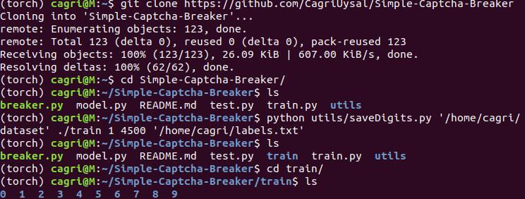
After cloning the repo, we can use saveDigits to create necessary traing folder which contains 9 distinct folder for each digit. It’s usage as follows:
python saveDigits.py <dataset-path> <train-digits-path> <startIndex> <endIndex> <groundTruth-path>
Here I used first 4500 images in the training (you can change the interval) and created train folder in the repo. If you are going to save the folder
in a different path, remember to change the root path in the train.py.
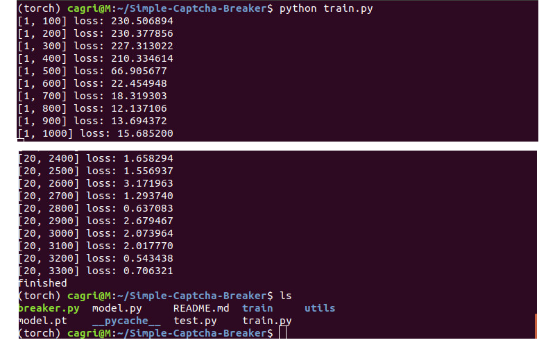
Once we have train folder, we can run train.py to train our model. You will see model.pt in the folder when the training finish.
Testing
Now it’s time to evaluate our model’s accuracy.
transform = transforms.Compose([transforms.Scale((24,14)),
    transforms.Grayscale(num_output_channels=1),
    transforms.ToTensor()])

dset = datasets.ImageFolder(root='test', transform=transform)
dloader = torch.utils.data.DataLoader(dset,
    batch_size=8, shuffle=True, num_workers=12)
test.py uses the same transformations as train.py and here only difference is, this time ImageFolder expects a folder named test.
As in the training part, we will create this folder using saveDigits.
total = 0
correct = 0

net = torch.load('model.pt').to(device)
with torch.no_grad():
    for i, (inp,lab) in enumerate(dloader,0):
        inp = inp.to(device)
        lab = lab.to(device)

        # forward pass
        outs = net(inp)
        # convert output scores to predicted class
        _, pred = torch.max(outs,1)
        correct += (pred == lab).sum().item()
        total += lab.size(0)

print('Accuracy: %f %%' % (100*correct/total))
In the above code, the trained model is loaded to net variable. Because we don’t need backprop while testing torch.no_grad is used to speed up computations.
The loop checks if the model predicts digits correctly and calculates the accuracy.
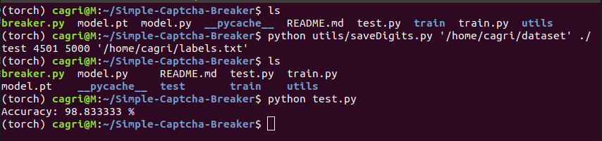
As in the training phase, we first created test folder using remaining images in the dataset. It is crucial to test the model
with data it has not seen before. This model achieves 98.8 percent accuracy.
The important thing to note here is achieved accuracy is per digit and not whole captcha. Thus single captcha has six digits inside, we can assume
0.988^6=0.93 of the time model will predict the whole captcha correctly.
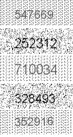
Using breaker.py we can break whole captchas. It’s usage as follows:
python breaker.py <image_file1> [<image_file2> ...]
Let’s give the first 5 test images and see the results.
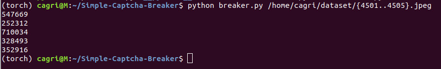
And that’s it. If you read this far I would like to thank you and I hope it has been helpful.
Cheers.